Linear Regression and Matrices
import pandas as pd
import numpy as np
import matplotlib.pyplot as plt
from scipy import stats
import statsmodels.api as sm
1 Load Data
Boston = pd.read_csv("../dataset/Boston.csv")2 Simple Linear Regression
The ISLR2 library contains the Boston data set, which
records medv (median house value) for \(506\) census tracts in Boston. We will seek to predict medv using \(12\) predictors such as rmvar (average number of rooms per house), age (average age of houses), and lstat (percent of households with low socioeconomic status).
Boston.head()| Unnamed: 0 | crim | zn | indus | chas | nox | rm | age | dis | rad | tax | ptratio | lstat | medv | |
|---|---|---|---|---|---|---|---|---|---|---|---|---|---|---|
| 0 | 1 | 0.00632 | 18.0 | 2.31 | 0 | 0.538 | 6.575 | 65.2 | 4.0900 | 1 | 296 | 15.3 | 4.98 | 24.0 |
| 1 | 2 | 0.02731 | 0.0 | 7.07 | 0 | 0.469 | 6.421 | 78.9 | 4.9671 | 2 | 242 | 17.8 | 9.14 | 21.6 |
| 2 | 3 | 0.02729 | 0.0 | 7.07 | 0 | 0.469 | 7.185 | 61.1 | 4.9671 | 2 | 242 | 17.8 | 4.03 | 34.7 |
| 3 | 4 | 0.03237 | 0.0 | 2.18 | 0 | 0.458 | 6.998 | 45.8 | 6.0622 | 3 | 222 | 18.7 | 2.94 | 33.4 |
| 4 | 5 | 0.06905 | 0.0 | 2.18 | 0 | 0.458 | 7.147 | 54.2 | 6.0622 | 3 | 222 | 18.7 | 5.33 | 36.2 |
To find out more about the data set, we can type ?Boston.
We will start by using the lm() function to fit a simple linear regression model, with medv as the response and lstat as the predictor. The basic syntax is {}, where y is the response, x is the predictor, and data is the data set in which these two variables are kept.
x = Boston['lstat']
y = Boston['medv']
2.1 Plotting Gotcha: Remember to Add/Remove Bias column
We calculate best-fit model by appending bias column to X but in plotting we need to remember to remove the bias column.
Convert_NPwill convert panda.Series to np.ndarrayX_bias: Will be used for plottingX: Input vectorlstatappended withbiascolumnbias: Column vector of 1’s- This allows us to get the Y-intercept or Beta_0 from linear regression
Convert_NP = lambda g: g.to_numpy().reshape(-1,1).astype('float32') #convert to one column ndarray
X = Convert_NP(x) #shape (560,1)
Y = Convert_NP(y) #shape (560,1)

X_NoBias = X #USED FOR PLOTTING PURPOSES


bias = np.ones((X.shape[0],1)).astype('float32') #column of 1's represent intercept coefficient
X_bias = np.append(X,bias,axis=1) #shape (560,2)
X = X_bias
print(f"X-dim: {X.shape}\nY-dim: {Y.shape}")
X-dim: (506, 2)
Y-dim: (506, 1)x_manual = np.linspace(Y.min()-Y.std(),Y.max()+Y.std(), Y.shape[0])
plt.scatter(X_NoBias,Y)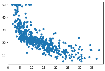
3 Manual
\[ \hat{\beta} = (X^T X)^{-1} X^T Y \]
Betas = np.dot(np.dot(np.linalg.inv(np.dot(X.T,X)),X.T),Y)
print(f"Betas: {Betas}")
Betas: [[-0.95004904]
[34.55383 ]]\[ \hat{Y} = X \hat{\beta} \]
medev \(=\) \(\beta_0 +\) \(\beta_1\)lstat
Y_hat = np.dot(X, Betas)  #shape (506,1)
x_manual = np.linspace(Y_hat.min()-Y_hat.std(),Y_hat.max()+Y_hat.std(), Y_hat.shape[0])
plt.scatter(X_NoBias,Y)
plt.plot(X_NoBias,Y_hat,color='g')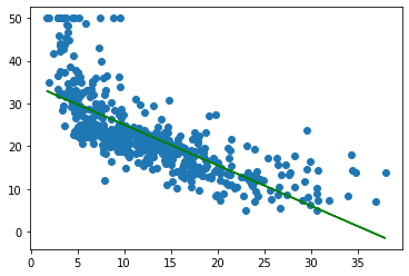
\[Residual = e_i = Y_i - \hat{Y}_i \tag{reducible error}\]
\[RSS = \sum_i (Y_i-\hat{Y}_i)^2 = \sum_i e_i^2\]
\[RSS = \sum Residual^2\]
\[MSE = \frac{1}{n} RSS \tag{loss function}\]
Residual = Y - Y_hat
RSS = (Residual**2).sum()
MSE = (1/Y_hat.shape[0])*RSS
assert RSS == ((Y-Y_hat)**2).sum()
print(f"Residual{Residual[:3]}\nRSS: {RSS}\nMSE: {MSE}")
Residual[[-5.822586 ]
[-4.27038 ]
[ 3.9748688]]
RSS: 19472.3828125
MSE: 38.482969985177863.1 prob-plot
Prob-plot is what ISLR actually uses but misleading labels QQ plot. QQ plot, plots againsts quantiles which are non-negative. We get these quantiles using the inverse CDF.
Prob-plot the theoretical quantiles is plotted on the x(Calculated using Filliben’s estimate) and our data’s z-score is plotting on the y.
Gotcha: Sort the x-axis of your Plot, REMEMBER TO USE PARAM axis=0
The x-axis, are the points that are divided into n-quantiles of the bell curve, n being the number of residuals you have.
This means that the area under the bell curve bounded between each of the n points are equal.
Know that since bell-curve is bigger in the middle means that there are denser points in the middle(less distance) and spread apart at each ends.
Z-score tells how many std-devs we are from the mean, can be positive or negative.
Quantile is equal area partition of probability density function.
CDF :: Z-score --> 100-Quantile, note that 100-quantile is just the percentile
InvCDF = stats.norm.ppf :: 100-Quantile --> Z-score
Resid_normed = Residual/Residual.std()

def Filliben(val):
    n = val.shape[0]
    fst = 1-(0.5**(1/n))
    midd = [(i-0.3175)/(n+0.365) for i in range(1,n-1)]
    lst = 0.5**(1/n)
return np.append(np.append(fst,midd),lst)Resid_normed.sort(axis=0)
print(np.append(Resid_normed[0], Resid_normed[1]))
InvertedPercentile = [stats.norm.ppf(i) for i in Filliben(Resid_normed)]
plt.scatter(InvertedPercentile,Resid_normed)[-2.4449956 -1.6037545]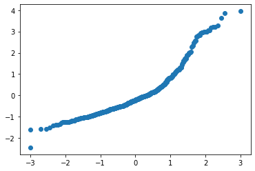
Residual_Standardized = Residual/Residual.std()
# notice the standardized residual is the z-score

normdist = np.random.normal( size=506)
print(Residual_Standardized.mean())
print(Residual_Standardized.std())
1.2740787e-06
1.0fig,ax = plt.subplots(2,2)
ax[0,0].scatter(Y_hat,Residual,facecolors="none",edgecolors="black")
ax[0,0].set_title("yhat vs e")
#yy = [stats.percentileofscore(Residual_Standardized, a, 'rank') for a in Residual_Standardized]
#yy2=np.sort(yy)
SortedResidStand = np.sort(Residual_Standardized,axis=0)
normdist = np.random.normal( size=506)
Sortednormdist = np.sort(normdist)
ax[0,1].scatter(Sortednormdist,SortedResidStand)
ax[1,0].scatter(Y_hat,np.sqrt(np.abs(Residual_Standardized)))
plt.show()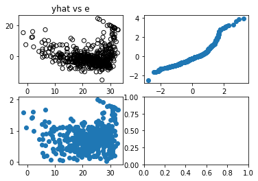
- yhat vs e(Top Left): used to check if there is a non-linear pattern
- The data point looks like a curve, clearly not linear
- Normal QQ Plot(Top Right): tells us if residuals fall in a normal dist if it fits the y=x diagonal
- the top part shows set of points above the y=x diagonal indicating heavy tails/ more chance of seeing extremes
- Scale-Location Plot(Bottom Left): tells us if residuals have non-constant variance (heteroscedasticity).
- If our data was linear, a constant variance would show a horizontal line pattern
- Since our data is not-linear, its hard to tell if the non-horizontal pattern is due to dynamic variance vs non-linearity
- Residual v Leverage Influence Plot(Bottom Right): Leverage points are outliers of the x-axis
- Leverage points should be removed
- Anything in Cook’s distance of 0.5 as shown by boundary is a leverage point to be removed
\[ Variance(\hat{Y}) = \sigma^2 = \frac{\sum_i (\hat{Y}_i-\overline{\hat{Y}}_i)^2}{n}\]
\[ TSS = \sum_i (\hat{Y}_i-\overline{\hat{Y}}_i)^2 \]
\[ Stddev(\hat{Y}) = \sigma\]
\[R^2 = 1-\frac{RSS}{TSS} \]
- TSS is just the numerator of Variance of Predictions
- TSS can be considered the background variance of our outputs Centered around the mean
- RSS can be considered variance between our datapoint Centered around the best-fit line
- RSS/TSS behaves like a normalized measure of how scattered or clumped our points are from our best-fit line.
Var_Yhat = ((Y_hat - Y_hat.mean())**2).sum()/Y_hat.shape[0]
Std_Yhat = Var_Yhat**0.5
TSS = ((Y_hat - Y_hat.mean())**2).sum()

assert np.isclose(Var_Yhat, Y_hat.var())
assert np.isclose(Std_Yhat, Y_hat.std())
\[SE(\hat{\mu}) = \frac{\sigma^2}{n}\]
- SE of sample mean tells us how far our sample mean is from population mean
SE_Yhat = (Var_Yhat)/Y_hat.shape[0]
print(SE_Yhat)0.090783711812010814 Statsmodels
model = sm.OLS(Y,X)
fit = model.fit()
print(fit.summary())
OLS Regression Results
==============================================================================
Dep. Variable: y R-squared: 0.544
Model: OLS Adj. R-squared: 0.543
Method: Least Squares F-statistic: 601.6
Date: Fri, 22 Apr 2022 Prob (F-statistic): 5.08e-88
Time: 10:33:30 Log-Likelihood: -1641.5
No. Observations: 506 AIC: 3287.
Df Residuals: 504 BIC: 3295.
Df Model: 1
Covariance Type: nonrobust
==============================================================================
coef std err t P>|t| [0.025 0.975]
------------------------------------------------------------------------------
x1 -0.9500 0.039 -24.528 0.000 -1.026 -0.874
const 34.5538 0.563 61.415 0.000 33.448 35.659
==============================================================================
Omnibus: 137.043 Durbin-Watson: 0.892
Prob(Omnibus): 0.000 Jarque-Bera (JB): 291.374
Skew: 1.453 Prob(JB): 5.36e-64
Kurtosis: 5.319 Cond. No. 29.7
==============================================================================
Notes:
[1] Standard Errors assume that the covariance matrix of the errors is correctly specified.fig,ax = plt.subplots(2,2)
pp = np.sort(Residual_Standardized,axis=0); # parameter axis=0 IS IMPORTANT!!
sm.qqplot(pp,line='45',ax=ax[0,1])
leverage = fit.get_influence().hat_matrix_diag
normresid = fit.get_influence().resid_studentized_internal
model_cooks = fit.get_influence().cooks_distance[0]
ax[1,1].scatter(leverage,Residual_Standardized)
ax[1,1].set_xlim(0,max(leverage)+0.01)
plt.show<function matplotlib.pyplot.show(close=None, block=None)>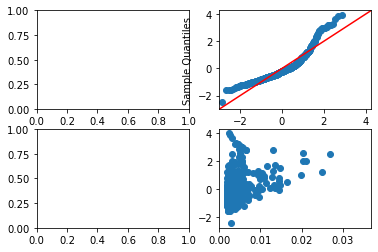
5 Scipy
result = stats.linregress(x,y)
print(f"""
Beta_1:\t\t{result.slope}
Beta_0:\t\t{result.intercept}
R:\t\t{result.rvalue}
R^2:\t\t{result.rvalue**2}
Beta_1 pvalue:\t{result.pvalue}
SE:\t\t{result.stderr}
Beta_0 SE:\t{result.intercept_stderr}
""")
Beta_1: -0.9500493537579908
Beta_0: 34.5538408793831
R: -0.737662726174015
R^2: 0.5441462975864798
Beta_1 pvalue: 5.081103394387796e-88
SE: 0.03873341621263941
Beta_0 SE: 0.562627354988433- MISSING
- Beta_0 pvalue
- tvalues for both Betas,
6 Numpy
Betas, RSS, Rank, SingVals =np.linalg.lstsq(X,Y,rcond=None)
print(f"""
Beta_1, Beta_0: {[i[0] for i in Betas]}
RSS: {RSS}
RSE : {(RSS/(X.shape[0]-2)) ** (0.5)}
Rank: {Rank}
SingularVal: {SingVals}
""")
Beta_1, Beta_0: [-0.95004934, 34.55384]
RSS: [19472.38]
RSE : [6.21576]
Rank: 2
SingularVal: [327.33368 11.027905]7 Torch
7.1 Simple LinReg
import torch
Xtensor = torch.from_numpy(X)
Ytensor = torch.from_numpy(Y)

W = torch.linalg.lstsq(Xtensor, Ytensor).solution
print(W)
# print(X[:,[1]])
Xlayer = torch.from_numpy(X[:,[0]])
hidlayer = torch.from_numpy(X[:,[1]])
Ytensor = torch.from_numpy(Y)
tensor([[-0.9500],
[34.5538]])7.2 1-layer NN
import random
import torch
from torch import nn, optim
import math
from IPython import display

device = torch.device("cuda:0" if torch.cuda.is_available() else "cpu")
seed = 1
random.seed(seed)
torch.manual_seed(seed)

inputDim = 1
outputDim = 1
hiddenDim = 100

learning_rate = 1e-4
lambda_l2 = 1e-6

model = nn.Sequential(
    nn.Linear(inputDim, hiddenDim),
    nn.Linear(hiddenDim, outputDim)
)
model.to(device) # Convert to CUDA

# nn package also has different loss functions.
# we use MSE loss for our regression task
criterion = torch.nn.MSELoss()

# we use the optim package to apply
# stochastic gradient descent for our parameter updates
optimizer = torch.optim.SGD(model.parameters(), lr=learning_rate, weight_decay=lambda_l2) # built-in L2

# Training
for t in range(1000):

    # Feed forward to get the logits
    y_pred = model(Xlayer)

    # Compute the loss (MSE)
    loss = criterion(y_pred, Ytensor)
    print("[EPOCH]: %i, [LOSS or MSE]: %.6f" % (t, loss.item()))
    display.clear_output(wait=True)

    # zero the gradients before running
    # the backward pass.
    optimizer.zero_grad()

    # Backward pass to compute the gradient
    # of loss w.r.t our learnable params.
    loss.backward()

    # Update params
    optimizer.step()
[EPOCH]: 999, [LOSS or MSE]: 39.632763plt.scatter(Xlayer.data.cpu().numpy(), Ytensor.data.cpu().numpy())
plt.plot(Xlayer.data.cpu().numpy(), y_pred.data.cpu().numpy(), 'r-', lw=5)
plt.axis('equal');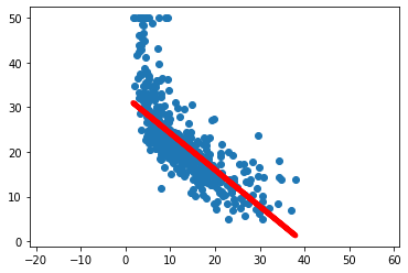
7.3 1 layer NN Class style
import torch
from torch.autograd import Variable
import torch.nn.functional as F

Xm = np.delete(X,1,1)
Xtensor = torch.from_numpy(Xm)
Ytensor = torch.from_numpy(Y)
numHiddenlayer = 1
#In pytorch we dont need to artifically add a hidden layer column to our X input
class LinearRegressionModel(torch.nn.Module):

    def __init__(self):
        super(LinearRegressionModel, self).__init__()
        self.linearA = torch.nn.Linear(Xtensor.shape[1], numHiddenlayer,bias=True)  # One in and one out
        self.linearB = torch.nn.Linear(numHiddenlayer,Ytensor.shape[1])
    def forward(self, x):
        #y_pred = F.relu(self.linear(x))
        y_pred = self.linearB(self.linearA(x))
        #y_pred = self.linearA(x)
        return y_pred

# our model
our_model = LinearRegressionModel()

criterion = torch.nn.MSELoss()

#EXTRREMELY SENSITIVE TO LEARNING RATE 1e-4 is sweetspot
learning_rate = (1e-4)

optimizer = torch.optim.SGD(our_model.parameters(), lr=learning_rate)

#w,b = our_model.parameters()
#print(f"initial: {w,b}")
bestloss = 99999
bestepoch = -1
for epoch in range(4000): #EXTREMELY SENSITIVE TO EPOCH, 50000 is sweetspot
    epoch += 1
    # Convert numpy array to torch Variable
    #inputs = torch.from_numpy(p).requires_grad_()
    #labels = torch.from_numpy(q)

    # Clear gradients w.r.t. parameters
    optimizer.zero_grad()

    # Forward to get output
    outputs = our_model(Xtensor)

    # Calculate Loss
    loss = criterion(outputs, Ytensor)
    currloss = loss.item()
    if currloss < bestloss:
        bestloss = currloss
        bestepoch = epoch
    # if currloss - bestloss > 200 and epoch > 50:
        # print("boom")
    # Getting gradients w.r.t. parameters
    loss.backward()

    # Updating parameters
    optimizer.step()

print('epoch {}, loss {}'.format(epoch, loss.item()))
print('epoch {}, loss {}'.format(bestepoch, bestloss))

#w,b = our_model.parameters()
#print(w,b)
epoch 4000, loss 38.486961364746094
epoch 4000, loss 38.486961364746094w,b = our_model.parameters()print(w,b)Parameter containing:
tensor([[-4.9096]], requires_grad=True) Parameter containing:
tensor([0.5459], requires_grad=True)8 Numpy vs Scipy vs Torch vs Statsmodels
From the above linear regression methods we can see that Numpy, Scipy, Torch lack the fine details that Statsmodel provide.
Statsmodel provide details that resemble R much more closely.