3d plots and Contour plot
Posted on October 15, 2021
Tags: codeetc
ax.contour3Dspecifically requires theaxsetup.plt.contourplt.contourfallows immediately plottingnp.meshgrid(x,y) = X,Ywhere X,Y are broadcasts of x and y to the same dimension- input x.shape is (2,1)
- input y shape is (3,1)
- rows of X are broadcasted copies of x
- X.shape is (2,3)
- cols of Y are broadcasted copies of y
- Y.shape is (2,3)
- Y.shape is (2,3)
- Notice that elementwise product of X and Y is the product space of x and y.
In other words, it is all combinations of x and y.
X,Y = meshgrid(x=[1,2],y=[3,4,5])
\[ x=\begin{bmatrix} {\color{red}1} & {\color{red}2} \end{bmatrix} \qquad y=\begin{bmatrix} {\color{blue}3} & {\color{blue}4} &{\color{blue}5} \end{bmatrix} \qquad X = \begin{bmatrix} {\color{red}1} & {\color{red}2} \\ 1 & 2 \\ 1 & 2 \end{bmatrix} \qquad Y = \begin{bmatrix} {\color{blue}3} & 3 \\ {\color{blue}4} & 4 \\ {\color{blue}5} & 5 \end{bmatrix}\]
\[X \otimes Y = \begin{bmatrix} (1,3) & (2,3) \\ (1,4) & (2,4) \\ (1,5) & (2,5) \end{bmatrix}\]
from mpl_toolkits import mplot3d
import numpy as np
import matplotlib.pyplot as plt
def cont3d(X,Y,Z,plottype="wireframe"):
fig = plt.figure()
ax = plt.axes(projection='3d')
if plottype == "contour3D":
ax.contour3D(X,Y,Z, 50, cmap='viridis')
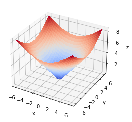
elif plottype == "surface":
ax.plot_surface(X, Y, Z, cmap="coolwarm", linewidth=0, antialiased=False)
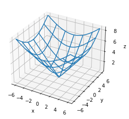
elif plottype == "wireframe":
ax.plot_wireframe(X, Y, Z, rstride=5, cstride=5)
ax.set_xlabel('x')
ax.set_ylabel('y')
ax.set_zlabel('z')
# ax.set_title('3D contour')
return (plt,ax)
def f(x, y):
    return np.sqrt(x ** 2 + y ** 2)

x = np.linspace(-6, 6, 30)
y = np.linspace(-6, 6, 30)

X, Y = np.meshgrid(x, y)
Z = f(X, Y)
print(X.shape,Y.shape)

fig,ax = cont3d(X,Y,Z,plottype="contour3D")
fig.show()
fig,ax = cont3d(X,Y,Z,plottype="surface")
fig.show()
fig,ax = cont3d(X,Y,Z,plottype="wireframe")
fig.show()
(30,)
(30, 30) (30, 30)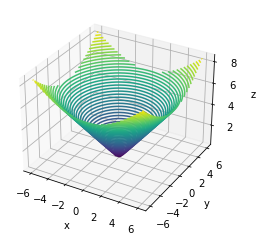
1 Simple Contour plots
- In 2d contour plots, color is the z-axis.
plt.contourf(X,Y,Z)<matplotlib.contour.QuadContourSet at 0x7fc419419910>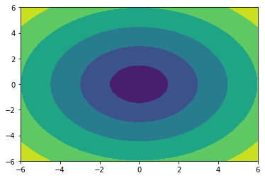
plt.contour(X,Y,Z)<matplotlib.contour.QuadContourSet at 0x7fc4192cc670>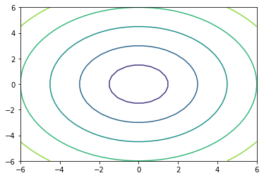
2 3d Plot
2.1 Plot random
def f(x, y):
    return np.random.poisson(size=x.shape)

x = np.linspace(-6, 6, 30)
y = np.linspace(-6, 6, 30)

X, Y = np.meshgrid(x, y)
Z = f(X, Y)

fig,ax = cont3d(X,Y,Z,plottype="surface")
fig.show()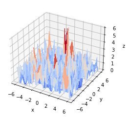
def f(x, y):
    return np.random.rand(*x.shape)

x = np.linspace(-6, 6, 30)
y = np.linspace(-6, 6, 30)

X, Y = np.meshgrid(x, y)
Z = f(X, Y)

fig,ax = cont3d(X,Y,Z,plottype="contour3D")
fig.show()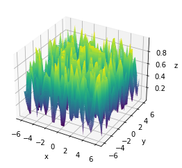
def f(x, y):
    return y

x = np.linspace(-6, 6, 30)
y = np.linspace(-6, 6, 30)

X, Y = np.meshgrid(x, y)
Z = f(X, Y)

cont3d(X,Y,Z)[0].show() 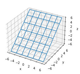
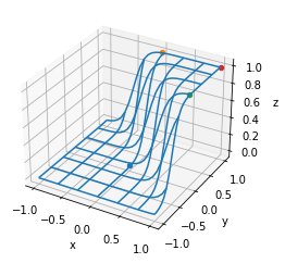
2.2 Manual Tuning Neural Net
| x1 | x2 | LinearFunc | Sigmoid | Actual x1 OR x2 |
|---|---|---|---|---|
| 0 | 0 | (0)(10)+(0)(10)+(-5)= -5 | σ(-5)=0.00669≅0 | 0 |
| 0 | 1 | (0)(10)+(1)(10)+(-5)= 5 | σ(5)=0.99330≅1 | 1 |
| 1 | 0 | (1)(10)+(0)(10)+(-5)= 5 | σ(5)=0.99330≅1 | 1 |
| 1 | 1 | (1)(10)+(1)(10)+(-5)= 15 | σ(15)=0.99999≅1 | 1 |
# Defina a collection of inputs to test OR and AND
my_x_collection = np.array([
    [0, 0],
    [0, 1],
    [1, 0],
    [1, 1],
])
def LinearFunction(x1,x2,w1,w2,b):
return (x1*w1 + x2*w2) + bdef Sigmoid_2d(x1, x2, w1, w2, b):
return 1/(1+np.exp(-LinearFunction(x1,x2,w1,w2,b)))- These are the weights we discovered, w1=10,w2=10,b=-5
w1 = 10
w2 = 10
b = -5print("Input\tLinear\tSigmoid")
for x in my_x_collection:
x1 = x[0]
x2 = x[1]
LinearOutput = LinearFunction(x1,x2,w1,w2,b)
SigmoidOutput = Sigmoid_2d(x1,x2,w1,w2,b)
print(f"{x}\t{LinearOutput}\t{SigmoidOutput}")Input Linear Sigmoid
[0 0] -5 0.0066928509242848554
[0 1] 5 0.9933071490757153
[1 0] 5 0.9933071490757153
[1 1] 15 0.999999694097773x = np.linspace(-1, 1, 30)
y = np.linspace(-1, 1, 30)
X, Y = np.meshgrid(x, y)
Z = Sigmoid_2d(X, Y, w1, w2, b)
fig,ax = cont3d(X,Y,Z)
ax.scatter(0,0,0)
ax.scatter(0,1,1)
ax.scatter(1,0,1)
ax.scatter(1,1,1)
fig.show()